4.1. Survey and monitoring techniques
4.1.1. Drilling, sampling, excavations
Modern NDT techniques continue to make road diagnostic surveys faster and more reliable, but they will never eliminate the need for drilling, boring and sampling. Structures will still need to be verified. NDT surveys will need calibration data and samples will need to be taken for laboratory analysis.


In surveys for the diagnosis of permanent deformation, samples for laboratory analyses should normally be taken from the base course. If it is thought that the rutting is related to a weak subgrade then samples should also be taken from the subgrade, or the subgrade soil type determined by an alternative method.

There are many techniques for verifying road structure thickness. The auger technique is still used in many countries but the main problem with the method is that the sample can be easily disturbed.

Other good methods include drilling or systems where a sampling tube is drilled or


hydraulically hammered through the road structure.


Excavation pits are also effective, especially if large numbers of samples are needed, but this technique can leave “ugly” patches in the pavement.


On many occasions the use of an excavator is the most reliable method to verify structures and the type of permanent deformation happening.


4.1.2.Visual inspections, videos, photos, thermal camera
Modern digital photo and video techniques provide some very useful tools for documenting a road and its surroundings:


Visual recording of the road, such as with a problem related to a blocked culvert, is vital for the correct diagnosis of the problem. Visiting, evaluating and documenting the actual site helps in locating problems and classifying the topography in the area.

The evaluation of drainage issues so far has generally been based on only visual inspections. A good visual documentation system can help external experts to become familiar with the specific problems at each location, even though they have not visited the site.
Digital video is the most useful and most rapidly increasing data collection technique today thanks to cheaper and higher quality cameras, higher capacity and cheaper computer hard drives, and better packing software.
Video recording gives a continuous record of the road. It can detect road surface condition, pavement distress, road markings, traffic signs etc. It can also be a very useful aid in surveying the topography of the road and its surroundings. A video recording of the road and ditches with an audio commentary is an easy way to gather basic information for a drainage analysis.
Video can be also used in the procurement process. A video recording, or a series of still photographs “before and after” the contract (or subcontract or measure), is a good way to evaluate the success of maintenance operations and monitor further work.
Video recording can be carried out simultaneously with other surveys, e.g. GPR and laser scanner measurements, and all data files can be linked together. They can also make a vivid presentation when gathered together.
A new very promising road survey technique, tested in the ROADEX project, is the use of modern high precision digital thermal cameras. The technique has proven particularly useful in drainage analysis associated with permanent deformation survey projects.

It can be used in pavement distress analysis together with traditional digital video. In some cases it can even detect cracks that are not visible on the top of the pavement.

In spring and early summer thermal camera surveys can also identify areas where frost is still present under the road.
 that can cause frost damages. This type of information can be useful in deciding the time when paving works can start after the winter.")

An even more useful feature is that the thermal distribution of the road surface can be obtained. This can give valuable information on any moisture anomalies in the pavement (e.g. due to pumping, cracking or poor drainage).
 and where the pavement has subsequently developed distress (right photo).")
4.1.3. Drainage evaluation
Permanent deformation hardly ever exists if the road structure and subgrade soils are kept free of excess water. Results from the ROADEX project clearly show that keeping the road drainage system in a good condition is the most profitable maintenance action that can be carried out on low volume roads. View: ROADEX II report: Drainage on Low Traffic Volume Roads and ROADEX III report: Developing Drainage Guidelines for Maintenance Contracts.
And the key to keeping the drainage working is an effective drainage monitoring system. A comprehensive drainage evaluation should preferably be carried out at the end of each maintenance contract period or at a maximum of 6 – 8 year intervals. Drainage evaluation has been traditionally done based on visual evaluation and digital videos, but recently laser scanning has also given excellent results. During the evaluation the problematic drainage sections can be identified and the need for improvement actions defined. After the problem drainage sections have been identified their condition should be checked every year. The results of the drainage analysis should then be saved into a database so the drainage information can remain available for future use.


A good drainage monitoring and improvement strategy can be divided into three phases:
- Phase 1. mapping the road sections suffering from inadequate drainage
- Phase 2. making a basic diagnosis of the drainage problem sites
- Phase 3. defining solutions for the problem sites
Phase 1: Mapping
The drainage analysis should be carried out on one road section at a time, and both sides of the road should be analyzed separately. Exceptionally, in those roads where the width is less than 5.5m, the inventory may be made in a single direction. During the data collection the speed of the survey vehicle should be between 20-30 km/h and vehicle should drive close to the pavement edge to give the cameras an unrestricted view of the ditch and side slope.

The surveyor should record the initial drainage condition class of the side ditch and outlet directly into the data collection laptop using the keyboard, and at the same time record any comments regarding the survey through the audio file of the digital video. Typically these comments should include:
- the classification of the drainage condition;
- the classification of the road profile;
- any corrections to the inventory which need to be corrected later;
- any observations on grass verges or pavement distresses that restrict water flow to the ditch;
- any notes on soil slippage from the inner and outer slopes to the bottom of the ditch, blocking the water flow.
These types of audio comments have been proven to be very valuable in ensuring the quality and repeatability of the inventory.

In addition to visual evaluation, laser scanner (lidar) and GPR techniques have been found to be excellent tools in drainage analyses. The laser scanner data can show the presence of verges and also ditch bottom levels. The GPR data can show the total thickness of the pavement structure which can be compared to the ditch bottom level. In addition recent innovations have shown that critical saturation levels can be calculated from the GPR data.


Phase 2: Diagnosis
The first action to be carried out in this phase is to establish a project for each road section surveyed where all of the data collected in the field can be linked to. This can be done, for example, with Road Doctor ® or similar software, where the initial drainage analysis results, crossprofile data, digital videos and still images can be linked to spatial data. Any road profilometer data (rutting and roughness) should also be linked to the project, preferably the last five years of historical data. This data can usually be abstracted from the road owner’s database or collected up-to-date on site. Once this has been done the final drainage analysis can be carried out using various techniques, depending on the type of coverage of the profilometer data. Either 10 metres or 20 metres average profilometer results should be used. Average results from 100 metres are too long on which to base a reliable drainage analysis. The correlation between pavement distresses and drainage condition should also be noted at this time.

.")


For gravel roads, the drainage analysis results should be compared with any spring thaw weakening inventory results and any distresses seen in the right-of-way road videos and still-images. A very good parameter to compare, if available, is the BCI-value calculated from the falling weight deflectometer (FWD). Comparison between frost heave and drainage can also be done, for example, by using IRI winter measurement results or antenna elevation data from a Ground Penetrating Radar measurement.
Phase 3: Solutions
Once the problem sections have been identified, and the locations recorded, the rehabilitation design can start. All data should be saved to an archive so that it can be accessed for the next, and future, drainage evaluations. By this means, monitoring and reviewing drainage condition in future years should be a simpler operation than the initial effort.


4.1.4 Pavement distress analysis – paved roads
What is pavement distress analysis?
Pavement distress analysis, as its name implies, can only be used to evaluate the type and extent of damage in the pavement layers of paved roads. Some indications of permanent deformation are also possible from a Pavement Distress Inventory (PDI). Earlier the most popular method to analyse pavement distress was a visual inspection made from a moving vehicle, but now different kinds of automated crack detection systems have entered to the market.
 should be analysed and classified according to their seriousness.")
Earlier pavement distress inventory (PDI), was normally used, as a semi-manual crack inventory methodology that is based on visual inspections made from a slowly moving vehicle. The driver of the vehicle tells the operator what kinds of cracks there are on the road and the operator enters the data on to a panel connected to a computer that feeds the survey information into a cracking database. The inventory is normally carried out on both lanes.

The road address and location of the vehicle should be automatically updated to the database. Video material can also be used as reference data. After the measurement is complete, various indexes describing the severity and the amount of distress can be calculated.

These types of visual inspection systems are, however, now considered to be unreliable and, for this reason, automated analysis methods are steadily gaining more popularity. They are also performed from a moving vehicle, but the measurement speed is much faster, usually no slower than the normal traffic speed. The vehicle can be equipped with digital video cameras, laser scanners or line scan cameras using either “picture interpretation” by computer software or laser-based measurement analysis.


In the “picture interpretation” system the software processes the picture data and detects any zones of deterioration. It can also generate maps that show the exact location of cracks. The laser scanner based system can measure rutting, unevenness and texture etc. The laser beams measure the road surface and create a model in which the deterioration zones can be seen together with the exact location of each zone.

Compared to the traditional PDI method, automated systems provide not only faster measurement speeds but better quality data, repeatability of measurements, information on the precise location of cracks, the possibility of integrating pavement distress analysis with other road condition measurements, and the possibility to develop new uses for the measurement data in the planning and procurement process.


The only disadvantage of the automated analysis method is that the system usually ignores occasional cracks in low deterioration zones and it is therefore important to always carry out visual inspections to validate the data.

Another very useful technique for pavement distress analysis is the thermal camera. This can be used in pavement distress analysis together with normal digital video. In some cases, the thermal camera can even detect cracks that are not yet visible on the top of the pavement. An even more useful output is the thermal distribution of the road. It can give valuable information on the moisture anomalies in the pavement such as due to pumping, cracking or poor drainage.

How pavement distress indicates permanent deformation?
There are a few “rules of thumb” that can be employed in evaluating pavement distress and deformation/rutting mode. In the case of net cracking (or “alligator cracking”), if the size of the nets is small and they are located only on the wheel paths, then the rutting mode is most likely to be Mode 1.


Narrow longitudinal “top down” type longitudinal cracks on both sides of the wheel path can also indicate Mode 1 rutting.
.")
Mode 2 rutting normally has bigger diameter net cracks than those of Mode 1, and cracking also appears outside the wheel paths.


In narrow roads longitudinal cracks between the wheel paths can also be indicators of Mode 2 rutting/deformation.


Where the drainage condition is poor, Mode 2 deformation can be also related to shoulder deformation and longitudinal cracking on the road shoulders.
4.1.5 Roughness, Rutting and Cross Fall Surveys
What is roughness and rutting?
Roughness and rutting are considered to be the most important parameters that affect the functional condition of a road and its service level.

Roughness means vertical unevenness on the road that can cause unhealthy vibrations in the human body. View the ROADEX III report “Health Issues Raised by Poorly Maintained Road Networks”. It generally consists of frost heave bumps, potholes and transverse and longitudinal cracks, to name a few, and is usually described using IRI (the International Roughness Index).
Rutting, on the other hand, is a result of uneven depressions in the pavement (and other layers) and can cause traffic safety problems, especially when the pavement is wet. These parameters, particularly the different indexes describing rutting, are very important indicators for permanent deformation.


The laser profilometer is a device that is used to measure roughness and rutting on paved roads. It can also measure the cross fall of the road. Many countries that measure roughness on gravel roads also use systems that utilize accelerometers.


Over recent years the use of laser profilometers in rutting measurements has been replaced by the laser scanner (lidar) technique. This technique provides a much higher point density than point lasers and thus results are more accurate and repeatable. Laser scanner based rutting survey data has also given much better understanding about the formation and root causes of deformations and especially how dynamic loading has an effect on rut formation.

The accelerometer is mounted on to the rear axle of the survey vehicle to give an indication of roughness under the wheel. Accelerometers are cheaper than laser profilometers and, thanks to their low price, will soon be generally adaptable to any passenger car, or public service vehicle such as a postal van, so that monitoring can be carried out on daily basis if needed.


An important issue in roughness and rutting surveys, and especially in analyses for permanent deformation on low volume roads, is that the data should be collected and analysed at short enough intervals to pick up local problems, i.e.. 5 m or 10 m. Structures and subgrade conditions, as well as drainage, can vary significantly on low volume roads over short intervals and longer data collection intervals can average out these values.

In addition to rutting and roughness, the cross fall and its changes have been found to be a very important parameter that can have a great effect on heavy vehicle accidents. Cross fall means the transverse slope of the road surface. On a straight section the centre of the road is generally higher than the shoulders. In curves, on the other hand, the outer shoulder should be higher than the inner one in order to improve the vehicle dynamics. Either way, it is very important that the road has sufficient cross fall, so that water can flow away from the road surface, and the drainage system can work properly. If the cross fall is inadequate, water may remain lying on the road and accelerate rutting. This can cause traffic safety problems.

 in the inner curve due to poor drainage and Mode 2 rutting leading to slope failure.")
How can roughness, rutting and cross fall data indicate permanent deformation?
It is not easy to identify if a road is suffering from permanent deformation, or a particular mode of rutting, from roughness data alone. ROADEX drainage survey results from the Rovaniemi maintenance area in 2006-2007 have shown that IRI is in general higher in places where the drainage condition is poor and the road is suffering from permanent deformation.
However, in these areas IRI values can vary greatly depending on how well the survey vehicle driver can follow the bottom of the ruts.

In frost areas, IRI values can be used to exclude frost related Mode 2 rutting.


Comparisons of different rutting measurement results can however be used to identify road sections suffering from permanent deformation.

For instance, a major difference between readings from “ridge” type rut depths and “PMS” type rut depths can indicate permanent deformation.

Another good indicator of permanent deformation is to monitor the increase in rutting rates (mm/year) on the road. Experience has shown that on paved low volume roads the road condition should be acceptable if the rut increase / year is less than 0.8 mm/year. Similarly, permanent deformation problems should be always suspected if the rut increase is higher than 1.5 – 2 mm/year.
 presented as a GIS map can indicate the location of problem places. This example is from road E10 in Sweden.")
 in Uusimaa area close to Helsinki, Finland. High rutting rates can be found in the high traffic volume roads due to studded tyres but they can also be found in low volume roads indicating permanent deformation problems.")
Road profilometer rutting trend analyses, and analyses of the cross fall of the road, can also provide valuable information where poor drainage is starting to trigger permanent deformation.

4.1.6 Laser Scanner Surveys
In recent years the greatest developments in NDT techniques for road surveys have been with laser scanners, and it is a fact that these systems will fast become a standard tool for the various tasks in the road condition management process.


Laser scanning is a technique where distance measurement is derived from the travel time of a laser beam from the laser scanner to the target and back. When the laser beam angle is known, and beams are sent to a range of directions from a moving vehicle with a known position, it is possible to make a 3D surface image, a “point cloud”, of a road and its surroundings. The point cloud can have millions of points, with every point having x, y & z coordinates and additional reflection or emission characteristics.
The accuracy of a laser scanner survey can be affected by factors that reduce visibility, such as dust, rain, fog or snow. High roadside vegetation can also prevent the capture of information from the hidden ground surface.
A laser scanner is composed of three parts: a laser canon, a scanner and a detector. The laser canon produces the laser beam, the scanner circulates the beam and the detector measures the reflected signal and defines the distance to the target. The distance measurement is based on the travel time of light, or phase shift, or a combination of both.
The quality and price of mobile laser scanner survey systems vary but they can be roughly classified into two categories:
a) effective high accuracy systems and


b) cheaper “everyman´s” laser scanner systems with reduced distance measurement capability and accuracy.

, a cross section of the road at the selected chainage (top right), and an emission map on the bottom.")
On low volume roads the laser scanner technique can be used in several applications. A road cross section can provide good information on the shape of rutting and if there are any verges preventing water flow away from the pavement.


A map of surface levels in colour codes has been an excellent tool in drainage analyses for finding those areas with poor ditches and clogged culverts. The changes in width of the road can also be easily seen from such maps.
 and cross section (top right) from a laser scanner survey, a drainage analysis (2nd field), rut depth information (3rd field) and a longitudinal profile of the road (4th field) showing the direction of water flow. This shows that the high permanent deformation at chainage 2025 is probably due to a blocked exit road culvert.")
A combination of laser scanner data together with other road survey data can provide an excellent basis for a permanent deformation analysis.
 together with a GPR radargram (2nd field), the dielectric value of the asphalt surface (3rd field) and FWD deflection bowls (lowest field). The data is from the ROADEX test site in Karrbäck, Sweden and the results show that the ditches have been filled almost completely which is causing water infiltration into the pavement structure and further permanent deformations.")
One more benefit of laser scanner point cloud data is that deformations can be viewed in the form of point cloud videos where road condition data can be presented together with surface data.

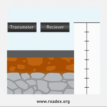
4.1.7 Ground Penetrating Radar (GPR)
What is Ground Penetrating Radar?
Ground Penetrating Radar (GPR) is a non-destructive ground survey method that can be used in researching roads, railways, bridges, airports, environmental objects, etc. Its main advantage is the continuous profile it provides over the road structures and subgrade soils and, as a consequence, the technique is becoming an increasingly important survey tool especially on the structural evaluation of low volume roads. A further, important advantage in road surveys is that it is not intrusive to other traffic using the road.

The method is based on transmitting short pulses of electromagnetic energy through materials using either an air coupled or

ground coupled antenna.


When an electromagnetic wave hits a boundary between substances with different dielectric constants, part of the wave reflects back to the surface and the antenna of the receiver picks it up. The rest of the wave either carries on to the underlying substance or scatters in multiple directions. The position and type of dielectric discontinuity of the materials can be indicated from the amplitude and frequency of the reflected pulses. GPR captures the data including the time (t) consumed in reflection and the amplitude (a).
GPR data must be processed with appropriate computer software in order to achieve understandable results.


Once the data is processed, one can interpret it in a number of ways, e.g. to calculate the thickness of pavement and road structure in general,
 used in thickness calculation.")
indicate problems in the road (e.g. ice lenses during frost season, Mode 2 rutting),

make approximate estimations of subgrade soils, locate peat and bedrock, etc.

There are many different electromagnetic wavelengths and antenna frequencies that can be used in GPR surveys depending on which layers are being surveyed. In pavement surveys, or surveys for the top part of the pavement structure, it is recommended that a high frequency (short wavelength) antenna is used because it can discriminate between thin layers. For high (1.0 – 2.5 GHz) frequency antennas the penetration depth is approximately 0.5 – 1.2 m and for lower frequency antennas (400 – 500 MHz) it is around 1.5 – 4.0 m. Low frequency antennas can only resolve thick layers, so the data is not necessarily as reliable as high frequency pavement data.


As a whole the accuracy of GPR method in thickness surveys is +/- 10 %. This can be improved to +/- 5 % if reference drill cores are available.

Even though data collection can be performed at maximum speed of 60 – 80 km/h it is recommended that for project level surveys, e.g. for permanent deformation evaluation, that the GPR survey should be carried out at a speed of 30 – 60 km/h to enable high quality video to be collected at the same time. Furthermore, due to the slower speed and more frequent sampling space (10 scans/m) the results can be more reliable.

In permanent deformation evaluations it is recommended that cross section profiles are also collected using GPR.


GPR systems are constantly developing and their use as a tool in road engineering is increasing. Third generation “3D” GPR systems with multiple antennas are now enabling better definition of rutting and permanent deformation modes.

Software packages for data processing and interpretation have also been strongly developing and many of them now allow linking and viewing GPS, maps and video data, together with GPR data making it easier to understand the problems with the road and its surroundings.

, 400 MHz (second field) GPR data, laser scanner rut depth data (third field) and TSD data (fourth field) shown together with digital video and point cloud rut depth video.")
How can GPR be used to identify permanent deformation?
There several ways that GPR data can be used to evaluate the type of rutting mode and permanent deformation causing problems to a road.
Mode 0 rutting: Mode 0 rutting normally takes place in a newly paved road. Problems with aggregate compaction can usually be seen in great variations of dielectric value of the pavement surface. This method can also be used as a quality control method to measure air voids content in pavement. Small variations in degree of compaction are however difficult to measure.

Mode 1 rutting: As discussed earlier, the main reason for Mode 1 rutting problems can usually be related to poorly performing base course materials. These materials can adsorb substantial quantities of water and this can be seen in GPR data as high dielectric values at the pavement-base course interface.

If FWD data is available, high SCI values or increased strain values, can confirm the GPR interpretation.
. The centre field shows the dielectric values of the base course in the left lane (red) and the right lane (blue) and the bottom field shows the pavement strains as measured by FWD.")
Mode 2 rutting: Mode 2 rutting can usually be seen in GPR cross sections as “onion like” reflectors in the road structures, and as thicker structures on wheel paths.

The “onion reflectors” can also be seen on longitudinal sections as multiple reflectors close to the road structure-subgrade interface.

“3D” GPR systems provide both longitudinal and cross section data, and this method is probably the easiest way of using GPR to identify Mode 2 rutting.

Finally, if FWD or TSD data is available, Mode 2 rutting can be confirmed with high BCI values or high deflection values measured at the geophone located 900 mm from the loading plate.

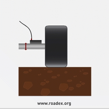
4.1.8. Dynamic Cone Penetrometer (DCP)
The Dynamic Cone Penetrometer is a “low-tech” device appropriate for evaluating the stiffness of road layers and subgrade that can also provide important information on road structures.
Its main component is the cone tip that is pushed (penetrated) into the ground by means of an 8 kg drop hammer.


The penetration depth for one or more drops is registered [in mm/drop] and the measurement is terminated when the cone reaches the planned depth or when the penetration rate after ten consecutive hammer drops is less than 3 mm/drop.
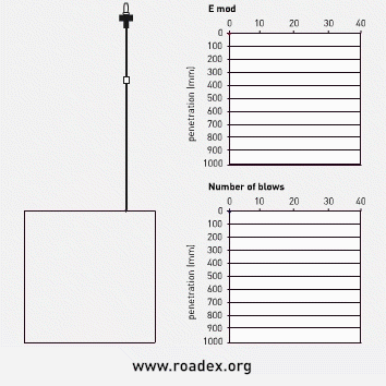
After the data has been gathered the survey results can be calculated to give CBR (California Bearing Ratio) or moduli values at each depth and, from these figures, the bearing capacity of the road can be estimated.


DCP can be used as a practical means of defining the thicknesses of road structures, shear strengths of road structures and subgrade soils, and to locate the frost line penetration depth. It is also possible to find relationships between DCP results and deformation features of the ground.

The DCP technique has some restrictions however, the greatest being that it cannot be used if the road structure material consists of large stones or boulders.


Often the DCP is used as a reference check for other survey methods and its use as a primary survey tool for low volume roads in the Northern Periphery requires further research. It is a useful tool however, especially in the exploration of spring thaw and frost lines.


4.1.9. Deflection measurements: Falling Weight Deflectometer (FWD), Light Weight Deflectometer (LWD) and Traffic Speed Deflectometer (TSD)
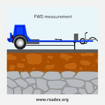
What is the Falling Weight Deflectometer
The Falling Weight Deflectometer (FWD) is an automated stationary impulse load method used to measure deflections in the road surface, which can then be used in calculating the bearing capacity of the road.
 equipment.")
 equipment.")
 equipment.")
FWD is usually based on a single axle trailer towed by a car and the measurements are automatically recorded so the driver does not need to leave the vehicle in order to carry out the measurements. The vehicle has to stop however for the actual measurement.
The device consists of a weight that drops from a pre-specified height on to a plate that is supported by rubber dampers that rest on a road-based circular plate with a specified diameter. The drop of the weight is designed to simulate the load produced by a passing heavy vehicle. The load applied to the road can vary from 20 to 150 kN, although the most common load is 50 kN on a 300 mm loading plate. The deflection is measured by multiple geophones placed radially starting from the centre of the load plate.
FWD is normally used for surveys on paved roads but it has also been successfully used in the Northern Periphery on gravel and forest road surveys. Besides bearing capacity measurement, the FWD, like all deflection measurements, can be used for many purposes, for example the investigation of reinforcement requirements, identifying weak spots of the road, establishing priorities for road strengthening, monitoring the strength of layers during construction, and of course research.

As a measuring method the FWD is rather slow, but it is the most common deflection survey method. In low volume roads the recommended data collection interval is 50 m.

Light Weight Deflectometer
On gravel roads, and on forest roads, another option for stiffness measurements in the FWD and DCP group is the portable Light Weight Deflectometer (LWD). This instrument measures the surface modulus, and some instruments have supplementary geophones that can help to identify if any bearing capacity problems are related to the layers close to the road surface.


Traffic Speed Deflectometer (TSD)
Over the last 10 years deflection measurement techniques from a moving vehicle have developed fast. The most popular technique has been the Traffic Speed Deflectometer technique, which uses laser doppler velocimeters to measure pavement response of a 10 ton trailer axle at a traffic speed of 5 – 80 km/h. From the deflection velocity the deflection under the wheel can be calculated. This is normally carried out at 5 m distances. The latest TSD versions enable deflection measurements also behind the wheel, which allows evaluations if the pavement response is elastic or visco-elastic. The benefits of TSD, compared to FWD systems, is that it collects data at traffic speed without any disruption to traffic flow and it simulates the impact of a real truck tyre. The continuous profile allows also precise diagnostics. TSD has proven to be very good in network level evaluations.
 truck measures pavement response under a real 10 ton trailer axle.")

, BCI (blue bars) and E2 (white bars) calculations. The fourth field presents bearing capacity calculated using the Odemark method. The fifth field gives the subgrade moduli values and the bottom the field pavement strains. The combined data shows a clear correlation between shoulder deformation and pavement strains.")
Deflection measurements and permanent deformation surveys
FWD data can be useful in a number of ways in permanent deformation projects. FWD parameters can help to identify the critical layer/depth with the highest risk for permanent deformation under the road surface, and it can also be used to calculate the parameters needed for dimensioning the new repair structure. However, it must be kept in mind, especially when evaluating base course materials and glacial till soils, that FWD readings measured from these materials can show quite high stiffness values if they are measured during dry summer months. So, if FWD data shows that material is poor, it is always poor. But if FWD data shows that material is good it can either be good or poor depending on when the FWD survey was carried out.

Back calculation of the layer and subgrade moduli values is the most common FWD evaluation method with asphalt pavements, especially in highly trafficked roads, but the method can also be used on low volume roads, and even on forest roads as this case from Scotland shows. In order to get reliable back calculation results, information on the layer thickness is needed and this is usually obtained from GPR data. When moduli values and thickness information of road structures and subgrade soils are known it is possible to calculate continuous surface bearing capacity for the whole road section using the Boussinesq-Odemark equation, and to evaluate those sections that have the highest risk for permanent deformation.


FWD and TSD data can also be used to calculate Surface Curvature Index (SCI) and Base Curvature Index (BCI) which can be very useful in determining whether a road has Mode 1 or Mode 2 rutting problems. The SCI is calculated by subtracting the D200 deflection value (or in some countries the D300 mm) from the D0 deflection value. This figure gives an indication of the stiffness of the pavement and the top part of the unbound base course. A high SCI value indicates a high risk for Mode 1 rutting.

The BCI is calculated by subtracting the D1200 deflection value from the D900 value and is an excellent indicator of how a road structures can spread a wheel load over a weak subgrade in order to reduce the vertical stress at the road structure / subgrade soil interface. If the BCI is high this indicates either Mode 2 rutting or pumping problems.

The recommended limit values for SCI and BCI values for paved roads, weak paved roads and gravel roads are given in the figure below.

The values shown for the “extremely poor” class have proven to correlate very well in predicting immediate pavement failures in low volume roads in Scotland and in Finland.
. The lowest field presents pavement roughness. Overall the combined data shows that high rutting and pavement strains correlate very well with high BCI values.")


4.1.10. Laboratory test methods
This lesson outlines the laboratory test methods recommended by the ROADEX project for detecting problematic road aggregates and diagnosing the underlying reasons for their poor properties. These materials are usually located in the base course or subbase layers of a road and are capable of reducing the pavement lifetime. The recommended laboratory tests can be divided in three stages.
Stage 1
The basic idea of the tests in Stage 1 is to run the most simple and cost-effective tests first, as sometimes these tests are enough in themselves to characterize the problem. The results of these tests indicate if material is moisture susceptible. They can however also give valuable information, if necessary, during the rehabilitation design process to select a proper treatment agent and technique to improve material quality. The recommended laboratory test methods during the first stage are a) grain size distribution analysis and b) organic content of the material. A further test c) water content of the material can also be determined (and is cheap to perform), but the result is very sensitive to errors, e.g. where samples have been improperly stored and the water content has been affected. A high gravimetric water content (> 5 % by weight) of the base material almost always indicates some kind of problem.

Grain size distribution is the most important factor in estimating the properties of problematic materials and should be analysed by the wet sieving method. The fines content and the shape of the particle size distribution curve will have an influence on the mechanical properties of the material and the results obtained can also give information for possible treatment options during the design stage. When ordering a grain size distribution analysis, it is important to remember to specify a “wet sieving” analysis as fine material can often become stuck on the surface of larger sized grains and these cannot be dislodged without water.

If the fines content after wet sieving is 10% or higher, the particle size distribution of the fines should also be determined. This can be done by using several methods, which can be based on sedimentation or laser diffraction.

The most common method, based on sedimentation, is the areometer method. This method is cheap, but slow, and the test normally takes a few days.

Once obtained, the results from the fines particle size analysis should be integrated with the results from the wet sieving test. When analysing these results, special attention should be given to the clay content (content of particles under size 0,002 mm). If the clay content of the whole material is higher than 3 %, then the analysed material is most likely to be frost susceptible and the road is likely to suffer from permanent deformation problems (Mode 1 rutting) during the thawing period or after freeze thaw cycles.

When analysing the grading curve of base material one should look first to the fines content, i.e. the relative amount of particles <0.063 mm. If the fines content is more than 10 %, the material will fail as a base course, even though the fines quality is good. In this case the particle size distribution of the fines should also be determined (see above). If the fines content is between 4-10%, the quality of the aggregate will depend on the quality of the fine material. If the fines content is less than 4%, the material is unlikely to have mechanical problems even though the quality of the fine material is poor. If the fines content is high (>5%) and the road has Mode 1 rutting problems, or other indications that can be related to poor quality base course material, it is recommended that additional tests should be performed before proceeding to Stage 2 in the analysis process.

Solutions for materials with high fines content can include the following: material treatment by bitumen or new treatment agents, “coarsening” (adding coarse material for instance ballast), or reducing the effective stresses on the material.
Another possible problem that can be seen with a grading curve is a high sandy fraction, evident as a “sand bag“ in the grain size distribution curve. This can also cause Mode 1 rutting.

Solution
In this case the best solution to improve the material quality is coarsening (adding open graded base or ballast).
Conversely, the grading curve can also show a lack of midsize grains. In this situation the grain size distribution curve is called “open graded“. If the material contains aggregates that are too coarse, it will be difficult to get an acceptable density during the initial compaction of the material, especially on low volume roads with weak foundations. This poor compaction can then cause Mode 0 rutting problems.

Solution
The solution in this case is to try to improve the compaction of the material. The good aspect of this type of rutting problem is that it reduces over time and in some case just a new pavement is enough. A further option is to add some sandy particles to the material.
It is common in many laboratories when making particle size distribution analyses to determine the organic material content as well. Organic material content can be defined, for example, by loss on ignition. High organic material content can cause moisture susceptibility, which can affect the selection of the treatment agent.

Stage 2
The goal of the laboratory tests in Stage 2 is to verify if the material is moisture susceptible. The most common tests used in this stage are a) the Tube Suction test, b) specific surface area of fines and c) water adsorption index test.
, specific surface area and water adsorption index.")
The ROADEX project recommends the Tube Suction test for the measurement of the water suction properties of road aggregates. This test measures if the aggregate adsorbs moisture when it is available in its surroundings. The amount of adsorbed water is monitored by measuring the dielectric value of the material at specified time intervals. The dielectric value is mainly a function of volumetric water content in the material. It is also recommended that the electrical conductivity of the material is measured during the Tube Suction test as this indicates the amount of osmotic suction in the sample, and if the material has problems, e.g. with chlorides.


The Tube Suction test is carried out in the following way. Before starting the test, samples are compacted into plastic tubes, 200 mm long and 150 mm diameter, and dried at +40-45 °C for at least 3-4 days before being left to stand at room temperature for at least 2 days. The bottoms of the dried samples are then placed in distilled water.

Dielectric values and electrical conductivity are then measured with a measuring device from the top of the sample at specified intervals (30 minutes, 1, 2, 4, 6, 8, 24, 32 hours and thereafter once a day from 2 days up to a minimum of 10 days until values have become steady). The magnitude and growth rate of the dielectric value reveals how much and how fast water rises to the top of the sample by capillary forces.

Unbound materials can be classified according to dielectric value. If the dielectric value is less than 9, the material will be a good quality for a base course material. If the dielectric value is 9-16, the material will be questionable as a base course material. If the dielectric value is more than 16, then the material will be inappropriate for use as a base course material.
If the electrical conductivity of the sample is high this means that the sample may contain high amounts of salts, or contain harmful weathering products from the aggregate minerals.
Solution
If the Tube Suction test results show that the material is questionable, or inappropriate as a base course material, the solution is to choose an appropriate treatment method or coarsen the aggregate. The tests in Stage 3 will be able to give some further information on the material and help to select a possible treatment method.

The specific surface area test indicates the surface area of the fine material. The bigger the measured area, the higher is the likelihood of water retention on the material particles. If the specific surface area is more than 4 000 m2/kg, it is a clear indication of some problems with the fines quality.

The water adsorption index indicates the potential for moisture to adsorb to the surface of the fine particles at 100% relative air humidity. It is also an indicator of how active the interaction is between the material and water. If the fines content is small (less than 4%) and the water adsorption index modest (<1 %), it is very unlikely that the analysed material is moisture susceptible and that moisture susceptibility is the reason for road damages. Adsorption values greater than 3% indicate some kind of problem if there are no chlorides in the sample. Water adsorption value is very sensitive to salt content and for this reason high water adsorption values should be always compared with electrical conductivity values from the Tube Suction test.

Stage 3
The laboratory tests in the third stage are special tests. These are the Proctor test, frost heave test and chlorides content.

If the laboratory tests in Stages 1 and 2 indicate that the material is moisture susceptible and that material treatment with stabilisation agents is possible, the Stage 3 test should be a standard Proctor test on the untreated material. The Proctor test gives an indication of the density of the compacted material at varying water contents. Compaction and mixing of most treatment agents on site are carried out near the optimum water content of the material. For this reason, the Proctor test is an important preliminary indicator of materials needing to be treated with stabilisation agents.

Frost heave tests are used to determine the frost susceptibility of materials. There are a number of different types of tests available but the constant temperature tests are the most commonly used ones.


Typically, the results of the frost heave test are presented as a function of time. Frost heave (h) is a clear parameter derived directly from displacement. Frost heave rate (v) refers to the frost heave over a unit of time and can thus be easily calculated from test results. Frost heave ratio indicates the ratio of frost heave (h) to the thickness of the frozen layer. The frost heave coefficient (SP), related to the segregation potential, is calculated as the ratio of the frost heave rate to the temperature gradient of the frozen sample section. If the frost heave coefficient is under 0,5 the material is not frost heaving. Slightly or extremely frost susceptible materials with high heave properties can be treated with suitable treatment agents.

When interpreting test results, it should always be kept in mind that the samples from road structures might have traces of contaminants, e.g. dust suppressant salts. If the material contains chlorides, these can have an influence on test results, for example the water adsorption index and electrical conductivity as measured in the Tube Suction test. Chloride content can be defined by a number of means, e.g. titration.

In addition to the laboratory test methods discussed in stages 1, 2 and 3 there is a further special test method that is often used to obtain the material parameters required for strengthening design, and that is the Triaxial test. The triaxial test is a useful test for determining the strength parameters of road materials, such as cohesion and angle of friction, that are needed for the ROADEX design approach against Mode 1 rutting.


The principle of the triaxial test is shown in figure. A cylinder-shaped sample is covered with rubber membrane and then put into a cell. The cell is pressurised, so that the sample experiences a triaxial stress state, and the sample very slowly compressed axially until it fails. The axial load is measured with a force sensor during the compression. A single test will give the shear strength of the sample in a particular stress state. A minimum of three tests are normally performed, using different cell pressures (stress state) for each sample.


The cohesion and the angle of friction can then be calculated on the basis of the tests.
 for each sample. The cohesion is the value of shear stress at the point where the line crosses the vertical axis. The angle of friction is the angle between the line and the horizontal axis.")


4.1.11. Integrated analysis of road survey results
All of the previous lessons should show that there is not one single method that can reliably solve all of the problems in permanent deformation diagnosis, or provide all of the information needed for good quality design. For this reason, it is important that a range of survey techniques should be used, and their combined results analysed at the same time in the office in an integrated fashion.

The best and easiest way to perform an integrated analysis is to view all the survey data on a PC screen using a modern software package specifically designed for the purpose. These types of packages allow the design engineer to compare survey results alongside digital videos and so evaluate whether the problems are related to particular circumstances or places. With these packages other specialists, such as geotechnical engineers, can become familiar with the specific problems at each location, even though they have not visited the site.

Integrated analysis can also permit the statistical analyses of a range of critical parameters in the diagnosis of permanent deformation. These include a) drainage class, b) thickness of the pavement and bound layers, c) total thickness of the road structures, d) subgrade soil type, e) road cross profile type and, as an example, f) if the problem spots are located in a straight road or on a curving section as a result of driving behaviour.
. The red area covers 90 % of the measurement points and the black line presents the median value. In this case the pavement condition is ok when the thickness, on average, is more than 50 mm.")
.")
The following case from Road 21 in Finnish Lapland provides a good example of the use of integrated road survey data and statistical analyses in the diagnosis of typical problems, and in getting useful information for rehabilitation design. In this case the GPR thickness data, FWD data and profilometer rutting data (ridge rut) were analysed together using a statistical analysis package.

The comparison between the FWD SCI values and the rutting median values shows that the higher the SCI value is the higher the rut depths are on the road. This relationship indicates that the main problem is likely to be Mode 1 rutting due to a poor-quality base course.

Comparison between the FWD BCI values and the different rutting levels tells us, on the other hand, that the BCI median value in the highest rutting class (>25 mm) is more than 40 µm. This indicates that there are also Mode 2 rutting problems in those sections with the highest rut depths.

Finally, a comparison of the pavement thickness values and rut depths suggests that a possible solution to the problem of the poor quality base course and Mode 1 rutting could be to use a total pavement thickness of 100 mm or more. This solution will not however work in areas with Mode 2 rutting problems and high BCI values and some other structural solution will be necessary for these areas.

4.2. Design for a project level survey system
The first task in a network or project level survey, is to collect and analyse all of the existing data available by making a site visit or interviewing local maintenance crews and, based on the results obtained, define the need for future surveys. View the ROADEX II report: Monitoring, communication and information systems & tools for focusing actions.

The selection of survey techniques to be used on a road section will depend on the type of road and the resources and techniques available. The recommended priority list of surveys for ROADEX projects is shown below. At least the first three surveys from this list should be always carried out, even when resources are minimal.
- A digital video of the road with GPS coordinates, or distance information.
- A distress analysis made during the data collection, or afterwards from the digital video.
- A drainage analysis made on site and/or from the digital video
- A GPR survey for a structural evaluation of the road
- A bearing capacity survey by FWD or TSD, or stiffness and structure thickness measurements by DCP Sampling and laboratory analyses
- Roughness and rutting surveys
- Laser scanner surveys
Data should not only be collected, it also needs to be analysed, and a decision should be made when planning a project on who is going to carry out the integrated analysis. Normally this will be the same person/consultant instructed to carry out the rehabilitation plan, but it can be also a separate person/consultant.
As stated earlier, a reliable positioning system is a key component of a successful monitoring and road survey project. This is obviously not a problem with a stationary monitoring system but with a mobile platform system positioning has to be done correctly. In a well-designed system this is often ensured through the use of double or triple systems, which means that the collected data is positioned using GPS data, DMI data (Distance Measurement Instrument, trip-meter) and digital video frame links. In such cases, the data collected can still be positioned correctly even though one system fails.

A common problem that arises when a number of road survey methods are used is a miss-match of the positioning referencing systems because of different trip meter calibrations, or different start points. For this reason, project managers should always ensure that all systems in the project use a common positioning system by marking the start and end points of the survey on the road with paint, or by fixed markers, etc.

4.3. Long term monitoring of low volume road structures
4.3.1. Monitoring trends
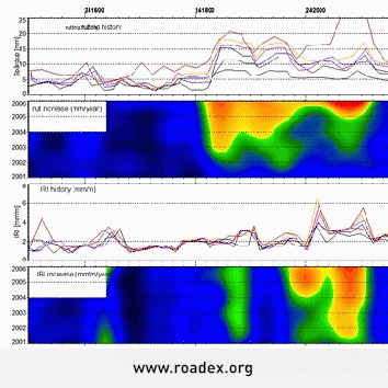
One of the most cost-effective ways for road condition management against permanent deformation is to monitor trends in the road behaviour. This means monitoring and analysing the road network as against time. For instance, when rutting is analysed on a road section as a rate of rut increase mm/year, this can immediately show those sections that are suffering from permanent deformation problems.

The information can also be used as a tool to guide preventative maintenance measures in the road. For example, analyzing the increase in rutting can identify areas with drainage problems at an early stage before any serious problems appear and when measures are easy and cheap to be carried out.
Trends can be calculated and monitored from several measurable road parameters. Those trends that can be monitored and give valuable information when managing against permanent deformation are:
, and later as measured roughness in the summer. This data presents different wavelengths calculated from accelerometer data.")
Rutting
If the rate of rutting increase on low volume roads is more than 0,8 – 1 mm/year permanent deformation should be considered. ROADEX recommends that a number of different ways of rut calculations and rut parameters should be used (such as the “PMS rut” and “ridge rut” in Finland, or distance between rut bottoms in Sweden). If a rutting rate increase is noticed, the first thing that should be done is to check the drainage condition. If the drainage is satisfactory a more detailed diagnosis will be required.


Roughness
Monitoring can identify quickly increasing roughness, due to frost fatigue problems or the development of rutting and pavement distress. The rate of increase of roughness can also indicate settlements problems, e.g. on road sections resting on peat. On good quality roads the IRI increase should be less than 0.5 mm/m/year. Problems generally start to appear where the IRI is more than 0.8 mm/m/year. Again, drainage should be checked first as a reason for any increased roughness. A good example of this is a blocked culvert that is seen in the smoothness of the road. If poor drainage is not the problem a more detailed diagnosis should be done.
.")
Pavement Distress: This indicator is likely to be very useful in the future for locating road sections suffering heavily from permanent deformation. The automated collection of a range of different parameters will allow an easier calculation of pavement distress.

Strain: Strain or asphalt moduli can be calculated from FWD or TSD data. FWD or TSD surveys should be carried out at least at 5 – 8 year intervals, and when measurements are taken on the same spots some comparisons can be made. An example of this can be seen when comparing Swedish Bearing Capacity Indexes on recently paved roads. On good road sections strains will stay fairly constant at a level of 200 or less, but in sections with Mode 1 deformation problems these strains can increase very quickly, up to a level to 300 – 400 microstrain, as the road approaches the end of its working life.

Dielectric values from a GPR air coupled antenna of the pavement surface or pavement base course interface can provide valuable information for road problem diagnoses. High dielectric values (>20) on gravel roads, and forest roads with a wearing course, can indicate drainage problems. High dielectric values can also indicate that the wearing course is adsorbing too much water and will be sensitive to permanent deformation and/or slipperiness during rain.
 with road drainage classes for both sides.")
Surface dielectric values can also provide information regarding the pavement condition of paved roads. On a newly constructed road the pavement surface dielectric should be normally between 5.0 – 7.0 with small deviation values depending on the mixture and aggregate type. After the first winter the value will increase slightly (roughly a value of one unit) and then stay stable if there are no problems. But when the water starts to break the bitumen-aggregate bonds, the pavement surface dielectric will start to increase. And when the cracking starts to appear on the pavement the deviation of the dielectric value will start to increase.


On paved roads, Mode 1 rutting should always be suspected if the dielectric value of the pavement/base course interface is higher than 9, or in Scandinavia even higher than 8.

Drainage and road shape
Extensive monitoring and trend analysis can be fairly expensive to carry out on low volume roads and are generally only recommended for high traffic volume roads, and on special weak low volume roads with high amounts of heavy traffic. Because of this it can sometimes be more profitable to perform a drainage analysis with a laser scanner, rather than a trend analysis, to define the critical sections that need special drainage maintenance.
and cross sections of a road measured using laser scanner technique.")

4.3.2. Monitoring seasonal changes
The ROADEX reports on spring thaw weakening and material properties have shown that the greatest amount (60 – 80 %) of rutting and permanent deformation takes place over the few days, or the few weeks, during the spring when the frost is thawing or, in non-frost areas, after a few frost nights followed by heavy rains. During the last few years however, due to global warming, the number of critical freeze-thaw cycles in early winter has increased dramatically across the Northern Periphery causing major problems to road owners, especially the forest industry.


In Northern Periphery countries the spring thaw weakening problem has traditionally been handled by applying load restrictions on the weak roads. This is cheap, and an easy way for road owners to handle the problem, but it does cause consequential problems to those local industries requiring heavy transport year-round. For this reason, the ROADEX project has been looking for new technologies to help solve the problems.View ROADEX II report: Managing Spring Thaw Weakening on Low Volume Roads.

A major problem however for road owners deciding if roads need load restrictions, or other measures to protect them from permanent deformation, is the general lack of information on seasonal changes in the road and its condition, and if it can carry heavy axle loads.
Due to the complex nature of permanent deformation resulting from seasonal change there are several critical parameters that should be monitored in a modern management system. These can be divided into three main categories: a) weather and temperature issues that can affect road structures and subgrade soils (freeze-thaw), b) moisture content, stiffness and the risk of permanent deformation, and c) information on heavy traffic. In an optimum system, all these categories should be monitored.

For the first category of weather and temperature, the most popular monitoring methods in the Northern Periphery for identifying whether road materials are frozen or thawed have been “frost depth“ and “soil temperature“ parameters. Previously these were monitored with “Gandahl tubes” installed in the road.

Now if the only goal is to monitor whether or not the road structures and soils are frozen, one of the best methods is to install temperature sensors at close vertical spacings in the road and subgrade soil.

Ground Penetrating Radar, especially when carried out in 3D, is also a useful tool for providing information on frost depth within a road, both in the longitudinal and transverse direction.


The second category of parameters consists of the engineering considerations, of which dielectric value is perhaps the most critical factor that should be measured when monitoring seasonal changes. The dielectric value is an indicator of volumetric free water content and, because it changes from a value of 81 to roughly a value of 4 when water freezes, the dielectric value can be used to determine if material is frozen.


Dielectric value can be measured using Time Domain Reflectometer probes (TDR)

and probes that detect changes in electrical capacitance. Capacitance based probes that also measure electrical conductivity and temperature have been successfully used in ROADEX field tests. The dielectric value of materials can also be monitored with the use of special Ground Penetrating Radar (GPR) sounding techniques. In recent years road engineers have been slowly moving from discussing water content in roads and materials to directly discussing the dielectric value itself.


Sensors can also be used to measure electrical conductivity and resistivity. These use the feature that soil becomes electrically resistive when it is frozen. It is worth noting with regard to electrical conductivity is that it can provide very valuable information about clay colloids and other matters during the thawing phase.

For instance, a period of surface thaw weakening, when the road surface is plastic, can be seen as a high peak in electrical conductivity readings.
 and electrical conductivity values (bottom) at the Kuorevesi Percostation during a spring thaw weakening period. The high peak in electrical conductivity indicates the time when road surface is plastic.")
The ROADEX II project has also shown that daily rainfall is an important parameter to monitor for the risk of road failures following freeze-thaw cycles. This is particularly the case in Scotland. In the future one parameter that has the potential to become very useful, especially on gravel roads, is evaporation.

Other important parameters, but more difficult and expensive to monitor, are parameters related to the stiffness of the road structures and subgrade soil (modulus and CBR). These can be measured using methods such as DCP, FWD and LWD that are described earlier in the lesson. The level of the road surface during frost heave and thaw settlement can also be useful parameters.

The final category of parameters concerns information on the heavy traffic using the road (even though this is outwith the direct monitoring of seasonal changes). The most common monitoring parameters here are the axle loads and total weights of heavy vehicles. These can be monitored with systems such as “Weigh In Motion” (WIM) techniques.
Results from the ROADEX II project show that the time intervals between heavy vehicles, and the road recovery times that follow, are very important parameters to consider when considering how to protect roads from damage during spring thaw. More information on recovery times will be given elsewhere in the lesson.

Despite everything that has been said however, it is still the case that the traditional way of monitoring spring thaw weakening, and seasonal changes is by visual inspection. The problem is that this is a very subjective, and relatively expensive, monitoring method and of the ROADEX partner countries only Finland has a formal systematic approach for visually monitoring spring thaw weakening damage and storing the information in databases.
